Not known Details About What Is Vlookup In Excel

Use VLOOKUP when you need to locate points in a table or a range by row. As an example, look up a cost of a vehicle part by the component number, or find an employee name based on their staff member ID. In its easiest type, the VLOOKUP feature says: =VLOOKUP(What you intend to seek out, where you intend to look for it, the column number in the range containing the value to return, return an Approximate or Precise suit-- indicated as 1/TRUE, or 0/FALSE).

Use the VLOOKUP feature to look up a worth in a table. Syntax VLOOKUP (lookup_value, table_array, col_index_num, [range_lookup] For instance: =VLOOKUP(A 2, A 10: C 20,2, TRUE) =VLOOKUP("Fontana", B 2: E 7,2, FALSE) =VLOOKUP(A 2,'Client Details'! A: F,3, FALSE) Debate name Summary lookup_value (needed) The value you wish to seek out. The worth you intend to seek out need to be in the first column of the series of cells you specify in the table_array argument.

Lookup_value can be a worth or a reference to a cell. table_array (needed) The variety of cells in which the VLOOKUP will browse for the lookup_value and also the return worth. You can make use of a called variety or a table, and you can utilize names in the disagreement rather than cell referrals.

The cell range additionally requires to include the return worth you intend to locate. Learn just how to pick varieties in a worksheet. col_index_num (required) The column number (beginning with 1 for the left-most column of table_array) that includes the return value. range_lookup (optional) A sensible worth that defines whether you want VLOOKUP to discover an approximate or a precise match: Approximate match - 1/TRUE assumes the initial column in the table is sorted either numerically or alphabetically, and will certainly then search for the closest worth.

For instance, =VLOOKUP(90, A 1: B 100,2, REAL). Precise match - 0/FALSE look for the specific worth in the initial column. For instance, =VLOOKUP("Smith", A 1: B 100,2, FALSE). There are 4 items of details that you will need in order to build the VLOOKUP phrase structure: The worth you wish to seek out, also called the lookup worth.

How To Use Vlookup In Excel - The Facts

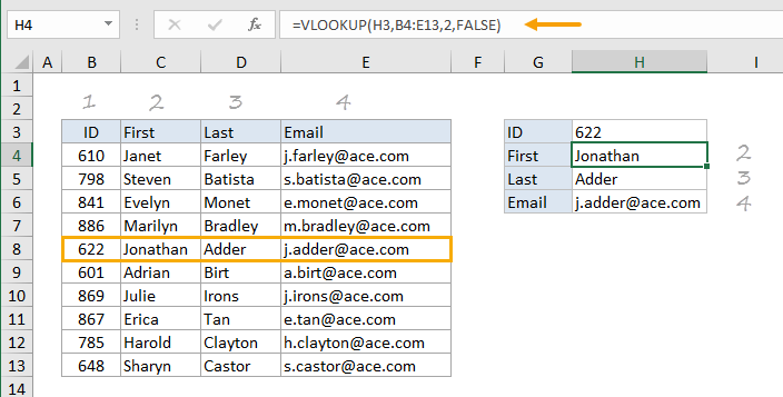
Keep in mind that the lookup worth ought to always be in the first column in the range for VLOOKUP to function correctly. For instance, if your lookup value remains in cell C 2 after that your range should begin with C. The column number in the array which contains the return worth. For instance, if you define B 2:D 11 as the variety, you need to count B as the very first column, C as the second, and more.

If you don't specify anything, the default worth will always hold true or approximate match. Now put every one of the above with each other as follows: =VLOOKUP(lookup value, array consisting of the lookup worth, the column number in the range having the return worth, Approximate match (TRUE) or Specific suit (FALSE)). Right here are a couple of examples of VLOOKUP: Issue What failed Incorrect value returned If range_lookup is TRUE or excluded, the very first column needs to be arranged alphabetically or numerically.

Either sort the initial column, or use FALSE for an exact match. #N/ A in cell If range_lookup holds true, after that if the worth in the lookup_value is smaller than the tiniest worth in the initial column of the table_array, you'll obtain the #N/ A mistake worth. If range_lookup is FALSE, the #N/ A mistake value suggests that the specific number isn't discovered.

#REF! in cell If col_index_num is higher than the number of columns in table-array, you'll get the #REF! error worth. For more details on dealing with #REF! mistakes in VLOOKUP, see Just how to remedy a #REF! mistake. #VALUE! in cell If the table_array is less than 1, you'll get the #VALUE! error value.

#NAME? in cell The #NAME? mistake worth generally means that the formula is missing quotes. To search for a person's name, make sure you make use of quotes around the name in the formula. As an example, go into the name as "Fontana" in =VLOOKUP("Fontana", B 2: E 7,2, FALSE). For even more details, see How to remedy a #NAME! error.

Not known Details About Vlookup Not Working

Discover just how to use outright cell referrals. Don't store number or day worths as message. When looking number or date values, make certain the information in the very first column of table_array isn't kept as text values. Otherwise, VLOOKUP might return an inaccurate or unforeseen value. Sort the very first column Kind the initial column of the table_array before making use of VLOOKUP when range_lookup holds true.

A concern mark matches any kind of solitary character. An asterisk matches any sequence of personalities. If you intend to discover a real concern mark or asterisk, kind a tilde (~) before the character. For instance, =VLOOKUP("Fontan?", B 2: E 7,2, FALSE) will certainly browse for all circumstances of Fontana with a last letter that might differ.

When browsing text values in the first column, see to it the information in the initial column doesn't have leading areas, trailing rooms, irregular use straight (' or") and curly (' or ") quotation marks, or nonprinting personalities. In these instances, VLOOKUP may return an unforeseen worth.

You can always ask a professional in the Excel Customer Voice. Quick Reference Card: VLOOKUP refresher course Quick Recommendation Card: VLOOKUP fixing tips You Tube: VLOOKUP video clips from Excel neighborhood professionals Every little thing you require to learn about VLOOKUP Just how to correct a #VALUE! mistake in the VLOOKUP feature Exactly how to correct a #N/ An error in the VLOOKUP function Summary of formulas in Excel Exactly how to stay clear of broken solutions Spot errors in solutions Excel functions (alphabetical) Excel features (by classification) VLOOKUP (cost-free sneak peek).

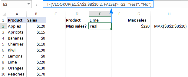
To compute delivery cost based on weight, you can make use of the VLOOKUP function. In the instance shown, the formula in F 8 is: =VLOOKUP(F 7, B 6: C 10,2,1)* F 7 This formula uses the weight to find the proper "expense per kg" after that ... To override output from VLOOKUP, you can nest VLOOKUP in the IF feature.

excel vlookup url vlookup in excel multiple sheets vlookup in excel userform